
In this post, I play with various plotting and visualisation options provided by base R, with a strong focus on small details.
Question 1
a)
1
2
3
4
5
6
7
8
9
10
11
12
13
14
15
16
17
18
19
20
21
22
23
24
25
# compute x and y for full distribution
x = seq(-4, 4, by=0.025)
y = dt(x, 20)
# get x and y of rejection region
rej_x = x[x >= 1.725]
rej_y = tail(y, length(rej_x))
# create plot
plot.new()
plot.window(xlim=c(-4, 4), ylim=c(0, 0.4), bty='n', yaxs='i')
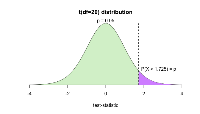
title(main='t(df=20) distribution', xlab='test-statistic')
# draw and fill distribution
lines(x, y)
polygon(x, y, border=NA, col=hcl(120, 50, alpha=0.5))
# draw and fill rejection region
lines(x=rep(1.725, 2), y=c(0, 0.4), lty='dashed')
polygon(c(1.725, rej_x), c(0, rej_y), border=NA, col=hcl(270, 230))
# add x axis and text
axis(1)
mtext('p = 0.05', side=3)
text(2.8, 0.1, 'P(X > 1.725) = p')

b)
1
2
3
4
5
6
7
8
9
10
11
12
13
14
15
16
17
18
19
20
21
22
23
24
25
26
27
28
29
30
31
32
33
34
35
36
37
38
39
40
41
42
43
44
45
46
47
48
49
50
51
# draw and fill a single rejection region
draw_rejection <- function(x, y, p, border, onesided) {
# dashed line at x
lines(x=rep(border, 2), y=c(0, 1), lty='dashed')
# fill between border and tail
polygon(c(border, x), c(0, y), border=NA, col=hcl(270, 230))
# add detail text
text(border*1.08, max(y)*1.1,
adj=ifelse(border < 0, 1, 0),
paste0('P(X ',
ifelse(border < 0, '<', '>'),
' ', border, ') = p',
ifelse(onesided, '', '/2')))
}
f <- function(df, p, onesided) {
# choose int x range limits based on some minimum p
xrange = round(qt(0.000125, df, lower.tail=F))
# compute x and y for full distribution
x = seq(-xrange, xrange, by=0.01)
y = dt(x, df)
# create plot
plot.new()
plot.window(xlim=c(-xrange, xrange), ylim=c(0, max(y)), bty='n', yaxs='i')
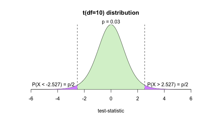
title(main=paste0('t(df=', df, ') distribution'), xlab='test-statistic')
mtext(paste('p =', p), side=3)
axis(1)
# draw and fill distribution
lines(x, y)
polygon(x, y, border=NA, col=hcl(120, 50, alpha=0.5))
# if not onesided, draw the left rejection region
if (!onesided) {
p = p/2
border = round(qt(p, df), 3)
rej_x = x[x <= border]
rej_y = head(y, length(rej_x))
draw_rejection(rej_x, rej_y, p, border, onesided)
}
# always draw the right rejection region
border = round(qt(p, df, lower.tail=F), 3)
rej_x = x[x >= border]
rej_y = tail(y, length(rej_x))
draw_rejection(rej_x, rej_y, p, border, onesided)
}
1
f(20, 0.05, TRUE)
1
f(10, 0.03, FALSE)
c)
1
2
3
4
5
6
7
8
9
10
11
12
13
14
15
16
17
18
# for reproducibility
set.seed(400)

# sample 30 from N(3,2) and compute t-statistics
n = 30
sample = rnorm(n, mean=3, sd=2)
means = seq(2, 4, by=0.5)
tstats = (mean(sample) - means) / (sd(sample) / sqrt(n))

# plot t-distribution with rejection regions
f(29, 0.05, F)

# overlay t-stat lines and labels
for (i in seq_along(tstats)) {
  lines(x=rep(tstats[i], 2), y=seq(0, 1))
  text(x=tstats[i], y=0.3, srt=-90, pos=4,
       labels=bquote(mu ~ '=' ~ .(means[i])))
}
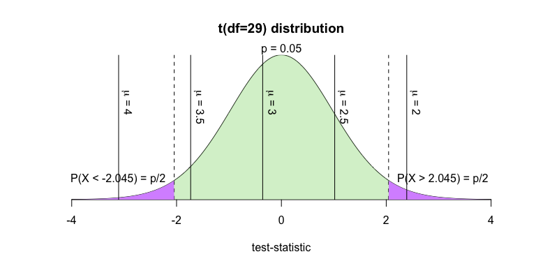
As illustrated above, μ = 2 and μ = 4 fall in the rejection region, indicating that the null hypothesis is rejected and the alternative is accepted given those mean values. The alternative hypothesis is not accepted for the other tested values of μ.
Question 2
a)
1
2
3
4
5
6
# read csv and separate year from month
imports <- read.csv('imports-by-country.csv')
imports$year = imports$yearmonth %/% 100
imports$month = as.integer(imports$yearmonth %% 100)
imports = subset(imports, select=-c(yearmonth))
head(imports)
1
2
3
4
5
6
7
##       country value year month
## 1 Afghanistan 60538 2000     1
## 2 Afghanistan 21641 2000     2
## 3 Afghanistan 28603 2000     3
## 4 Afghanistan 34781 2000     4
## 5 Afghanistan  3130 2000     5
## 6 Afghanistan 11199 2000     6
1
2
3
4
5
# list the top three countries by total value of imports
country_sums <- aggregate(value ~ country, imports, sum)
sorted_country_sums <- country_sums[order(-country_sums$value),]
top_three_countries <- head(sorted_country_sums, 3)
top_three_countries
1
2
3
4
##                         country        value
## 43  China, People's Republic of 157224053406
## 12                    Australia 153492831803
## 233    United States of America 105147208043
b)
1
2
3
# draw a pie chart of total imports from each country
with(sorted_country_sums,
     pie(value, labels=country, main='Proportion of imports to NZ since 2000'))
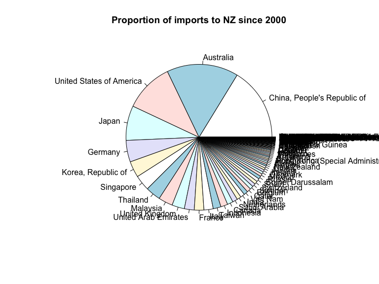
There are too many countries listed in this visualisation, so I would prefer to bin the smallest into an “other” group or narrow the range of countries listed.
The default colors used in this visualisation repeat, which may cause the viewer to wrongly associate unrelated countries.
c)
1
2
3
4
5
6
7
8
9
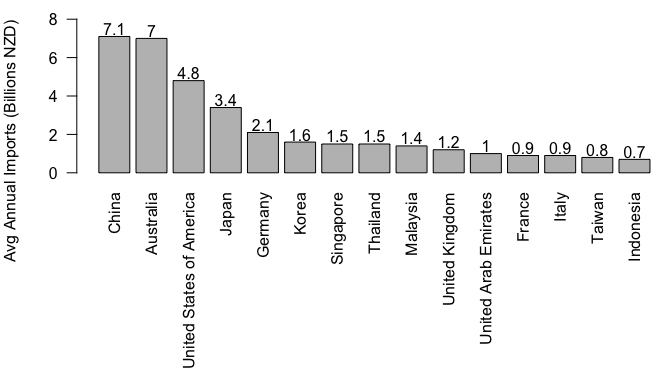
# get top 15 countries by average annual imports
annual_imports <- aggregate(value ~ country + year, imports, sum)
avg_annual_imports <- aggregate(value ~ country, annual_imports, mean)
sorted_avg_imports <- avg_annual_imports[order(-avg_annual_imports$value),]
# convert values to billions NZD and show
sorted_avg_imports$value <- round(sorted_avg_imports$value / 10^9, 1)
top_annual <- head(sorted_avg_imports, 15)
top_annual
1
2
3
4
5
6
7
8
9
10
11
12
13
14
15
16
##                         country value
## 43  China, People's Republic of   7.1
## 12                    Australia   7.0
## 233    United States of America   4.8
## 110                       Japan   3.4
## 85                      Germany   2.1
## 115          Korea, Republic of   1.6
## 192                   Singapore   1.5
## 217                    Thailand   1.5
## 130                    Malaysia   1.4
## 231              United Kingdom   1.2
## 230        United Arab Emirates   1.0
## 77                       France   0.9
## 108                       Italy   0.9
## 214                      Taiwan   0.8
## 103                   Indonesia   0.7
1
2
3
4
5
6
7
8
9
# remove 'republic of' from country names
cnames <- sapply(strsplit(top_annual$country, ','), `[`, 1)

# barplot the top 15 countries
par(mar=c(11,4,1,0))
mybar <- barplot(top_annual$value, ylim=c(0, 8),
                 names.arg=cnames, las=2)
text(mybar, top_annual$value+0.4, top_annual$value)
title(ylab='Avg Annual Imports (Billions NZD)', adj=1)
d)
1
2
3
4
5
6
7
8
9
10
11
12
13
14
15
16
17
18
19
20
21
22
23
# ---- DATA PROCESSING ----
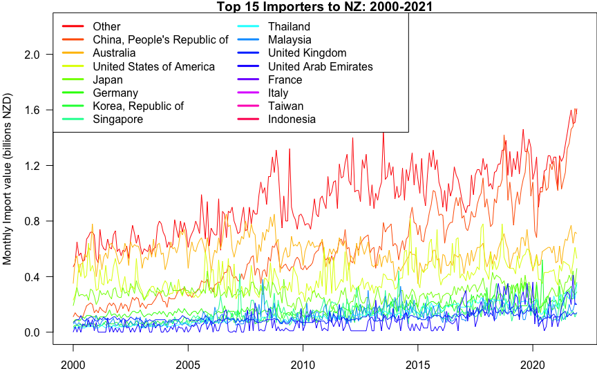
# get monthly imports of top 11 by avg annual imports
top_eleven <- head(sorted_avg_imports, 11)
top_monthly <- subset(imports,
country %in% top_eleven$country)
# sum up monthly imports of all other countries
all_others_monthly <- subset(imports,
!(country %in% top_eleven$country))
other_monthly <- aggregate(value ~ year + month,
all_others_monthly, sum)
other_monthly$country <- 'Other'
# combine top 11 with 'other' and sort by time/date
monthly <- rbind(top_monthly, other_monthly)
monthly$time <- as.Date(with(monthly,
paste(year, month, '01', sep='-')))
monthly <- monthly[order(monthly$time),]
# convert monthly imports to billions and show sums to confirm
monthly$value <- round(monthly$value / 10^9, 2)
aggregate(value ~ country, monthly, sum)
1
2
3
4
5
6
7
8
9
10
11
12
13
##                        country  value
## 1                    Australia 153.48
## 2  China, People's Republic of 157.23
## 3                      Germany  46.17
## 4                        Japan  74.43
## 5           Korea, Republic of  34.72
## 6                     Malaysia  30.59
## 7                        Other 251.72
## 8                    Singapore  33.33
## 9                     Thailand  32.37
## 10        United Arab Emirates  21.12
## 11              United Kingdom  26.91
## 12    United States of America 105.07
1
2
3
4
5
6
7
8
9
10
11
12
13
14
15
16
17
18
19
20
21
22
23
24
25
26
# ---- PLOTTING ----

# merge sorted country names to create palette
countries <- c('Other', top_annual$country)
cols <- rainbow(length(countries))

# create plot
plot.new()
par(mar=c(2,4,1,0))
with(monthly,
     plot.window(xlim=c(min(time), max(time)), ylim=c(0, max(value)+0.6)))
box()

# plot a line for each country's monthly imports
for (i in seq_along(countries)) {
  country_imports <- monthly[monthly$country==countries[i],]
  with(country_imports,
       lines(time, value, col=cols[i]))
}

# add title and axes
title(main='Top 15 Importers to NZ: 2000-2021',
      ylab='Monthly Import value (billions NZD)')
axis.Date(1, monthly$time)
axis(2, at=seq(0, 2, by=0.4), las=2)
legend('topleft', legend=countries, col=cols, lty=1, lwd=3, ncol=2)
e)
1
2
3
4
5
6
7
8
9
10
11
12
13
14
15
16
17
18
19
20
21
22
23
24
25
26
27
28
29
30
31
32
33
34
35
36
37
38
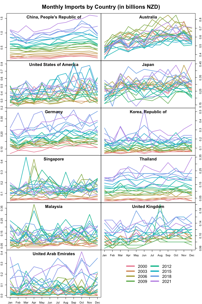
# drop 'Other' from countries
m <- monthly[monthly$country!='Other',]
co <- top_eleven$country
# create year range and color palette
years <- 2000:2021
legend_inds <- seq(1, length(years), by=3)
angles <- (seq_along(years)-1)/length(years)
cols <- hcl(h=angles*300, c=60, l=70)
# create layout and loop through countries
par(mfrow=c(6,2), mar=rep(0,4), oma=c(2,2,4,2), cex.main=1.5)
for (i in seq_along(co)) {
# get monthly imports of this country
c.df <- m[m$country == co[i],]
# create new plot
plot.new()
plot.window(xlim=c(1, 12), ylim=c(min(c.df$value), max(c.df$value)))
box()
# draw a line for each year of imports
for (j in seq_along(years))
with(c.df[c.df$year == years[j],],
lines(month, value, col=cols[j], lwd=2))
# add title and draw axis if left/right/bottom edge
title(main=co[i], line=-1.5)
if(i %% 2 == 0) axis(4) else axis(2)
if(i > length(co)-2) axis(1, at=1:12, labels=month.abb[1:12])
}
# add legend in final plot space and top title
plot.new()
legend('center', legend=years[legend_inds], col=cols[legend_inds],
cex=1.5, ncol=2, lty=1, lwd=5, bty='n')
par(cex.main=2)
title(main='Monthly Imports by Country (in billions NZD)', outer=T)
f)
Based on the above figure, imports from Australia have a clear seasonal pattern. Each year consistently bottoms out in January and climbs to a peak in December, likely due to the timing of winter holidays around the New Year.
The above plots also illuminate steadily increasing imports from nations like China and Thailand. The warm hues of earlier years are consistently lower than the cooler hues of later years’ lines, reflecting a steady increase in imports each year.